You're still using VLOOKUP?!

Did You Know? 100% of people who use VLOOKUP are wrong. (Source: Me.)

Who’s ready for some spreadsheet fun!

Today, we’re talking about lookup functions.

Specifically, we’re comparing these 3:

• VLOOKUP

• XLOOKUP

• INDEX-MATCH

My goal: To show you why INDEX-MATCH is the undefeated champion of the lookup function world.

I’ll be using this Google Sheet with a pre-filled example, in case you want to follow along.

Here’s our situation.

Tim’s Tiny Top Hats

Today, you’re a marketing analyst for Tim’s Tiny Top Hats, a company that sells tiny top hats for dogs.

Why?

I’ll tell show you why.

Tim tasked you with analyzing the performance of 2023’s monthly email marketing campaigns to calculate two data points:

• Revenue generated per 1,000 sent emails

• Revenue generated per 100 clicks

You have two sets of data.

Email marketing data from your email marketing tool:

Website analytics data from your website analytics tool:

Both datasets have unique keys of “ID” and “Month” by which you can join them to create an aggregated table with all of the fields needed to calculate the metrics Tim needs.

When you’re done, your new table looks like this (keeping only the fields needed for your calculations):

Nice work!

Let’s look at how you could have accomplished this task using each of the 3 different lookup functions.

Note 1: This example assume you know that “$” can be used in a formula to “fix” a cell reference and make it unchangeable. Although, if you didn’t know that, I guess you do now. No assuming necessary!

Note 2: These functions all have optional terms that can be confusing to explain. I’ll only include the optional terms you’ll need for this exercise, so don’t worry about all of the optional stuff unless I explicitly tell you to start worrying about it.

Method 1: VLOOKUP

VLOOKUP is objectively the worst way to approach this task. That’s not an opinion. It’s just a fact.

Here’s the VLOOKUP function and what each of its terms mean:

=VLOOKUP(lookup_value, table_array, col_index_num, [range_lookup])

There are 3 required terms and one optional term.

• lookup_value: Value you want to use as your lookup key

• table_array: Range of cells containing all of your data, including both the lookup_value and the value you want to return

• col_index_num: Column number in the table_array containing the final value you want to return.

• [range_lookup]: (Optional) TRUE or FALSE, whether you want the formula to return an exact match for your lookup_value. You almost always want FALSE, which specifies an exact match

Let’s look at how we can use VLOOKUP to build our aggregated table.

In image below, we’re trying to add email “Sends” counts for each of the “Month” values in column B.

This is the formula we’re using:

• $B$18 specifies “January” as the term to search for.

• $B3:$H14 defines the range for the entire email marketing table, starting with the column where “lookup_value” exists.

• 3 identifies “Sends” as being the 3rd column in “table_array”

• false specifies an exact match, meaning we want to look for an exact match of “January” in column B.

That seems all well and good, but the problem is VLOOKUP’s lack of flexibility. Here’s how we need to look up the values of our 4 fields—Sends, Clicks, Sales, and Revenue—across the 2 tables for all 12 months:

We need to use 2 different table arrays (1 for the email marketing table and 1 for the web analytics table) and 4 separate hard-coded column index numbers.

If the structure of our tables change, those hard-coded column indices now are referencing the wrong columns, which means our aggregated table breaks.

Method 2: XLOOKUP

XLOOKUP is leagues better than VLOOKUP, mostly because it’s more flexible when the column containing the data you want to return changes its position in your array (this happens when you add or remove columns from a table).

Here’s the XLOOKUP function and what each of its terms mean:

=XLOOKUP(lookup_value, lookup_array, return_array, [if_not_found], [match_mode], [search_mode])

There are 3 required terms and 3 optional terms (none of which we need for this exercise):

• lookup_value: Value you want to use as your lookup key

• lookup_array: Range where the function will search for your lookup_value

• return_array: Range where the function will search for the corresponding value to return

Like VLOOKUP above, let’s look at how XLOOKUP references the “Sends” field for our new aggregated table:

It’s essentially the same idea as VLOOKUP’s approach, except XLOOKUP replaces the hard-coded column index number (“3” for “Sends”) with the reference range (“$B$3:$B$14” for “Sends”). This makes XLOOKUP resistant to column additions/deletions, as the column reference will change as needed.

XLOOKUP, though better than VLOOKUP because the column indices are ranges instead of hard-coded values, still suffers from the complexity of having 4 separate formulas—one for each of Sends, Clicks, Sales, and Revenue.

If all of our columns are next to each other in the same table, we can just use “$” to fix the proper columns or rows and then drag the formulas across, but that isn’t the setup we have here.

• Sends and Clicks are in columns D and F from the Email Marketing table with column E (Opens) separating them.

• Sales and Revenue are in columns N and P from the Web Analytics table with column O (Avg Order Value) separating them.

Thus, we still have a disjointed formula setup in our aggregated table where we can’t just write a single formula and drag it across all cells.

INDEX-MATCH solves this problem.

Method 3: INDEX-MATCH

INDEX-MATCH is my go-to lookup function 100% of the time. It can be as simple or as complex as you need it to be, so I don’t see a need to ever use VLOOKUP or XLOOKUP.

That said, there are two potential downsides to INDEX-MATCH:

1. The syntax is a little more confusing, because it requires nested formulas.

2. It’s less common than either VLOOKUP or XLOOKUP, so it isn’t as team-friendly when working in files that multiple people maintain. (Unless you convert everyone!)

INDEX-MATCH is made by combining two separate functions: INDEX and MATCH.

MATCH is nested inside INDEX, so we’ll start there.

MATCH Function

What MATCH Does: MATCH looks for the position of a value in either a single row or single column.

Here’s what MATCH looks like.

=MATCH(lookup_value, lookup_array, [match_type])

There are 2 required terms and 1 optional term, which we do need:

• lookup_value: Value you want to use as your lookup key

• lookup_array: Range where the function will search for your lookup_value

• [match_type]: (Optional) Whether formula should return exact or approximate match; accepts 0 (exact match), 1 (largest value less than or equal to lookup_value), or -1 (smallest value greater than or equal to lookup_value)

INDEX Function

What INDEX Does: INDEX starts with an array (basically, a table with multiple rows and columns) and returns a value for a single pairing of row and column number.

Here’s what INDEX looks like:

=INDEX(array, row_num, [column_num])

There are 2 required terms and 1 optional term, which we do need for this task:

• array: Range of cells from which you want to retrieve a value

• row_num: Row number where the return value exists in the array

• [column_num]: (Optional) Column number where the row value exists in the array

Here’s how the two work together.

INDEX-MATCH Function

INDEX-MATCH is a nested formula with MATCH inside INDEX. This is the general approach:

• INDEX takes an entire table and returns the value for the provided row and column numbers.

• MATCH provides the row and column numbers by determining where the lookup values are in a provided range.

Putting them together, we’re doing this:

=INDEX(range_both_tables, MATCH_TO_GET_ROW, MATCH_TO_GET_COLUMN)

Here’s what our formula looks like to return “Sends” for “January” just as we’ve done with VLOOKUP and XLOOKUP:

Let’s break each of those terms down one at a time.

Term 1: Range spanning both tables

The first term defines the range where all of our values are located. In this example, that’s the range from $A$2:$P14, which contains all of the data for both tables.

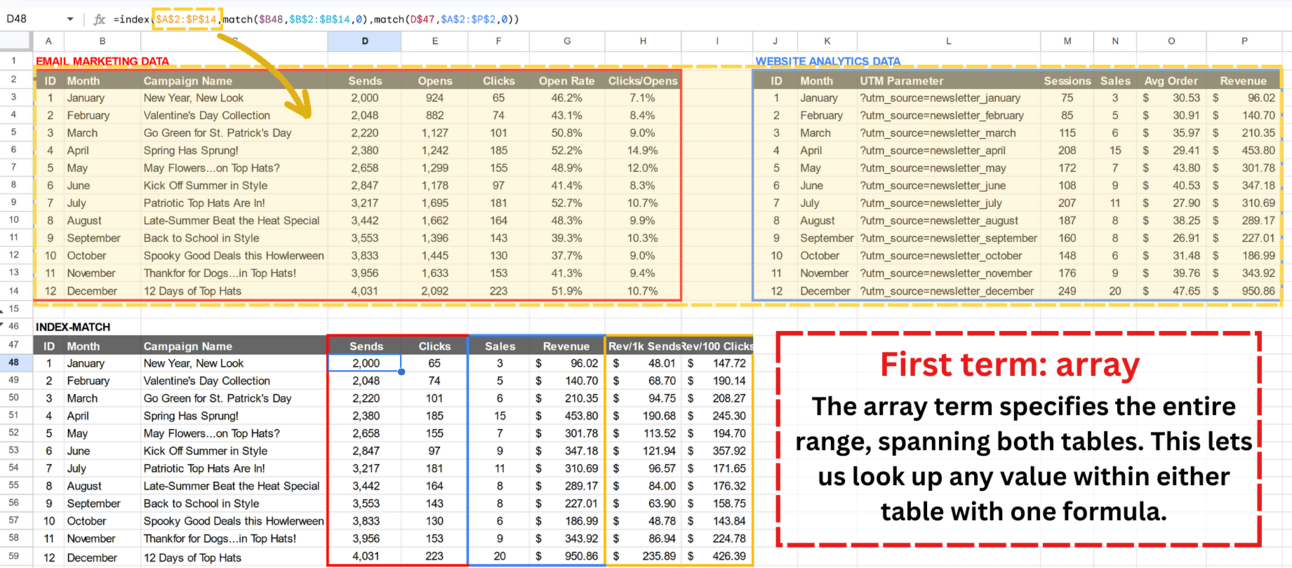
Term 2: Lookup which row contains the month we want “January”

The second term defines the row containing the value we want. Because we want “Sends” for the month of “January”, we’re looking for where “January” (cell $B48) exists in the range of months ($B$2:$B$14) in our two-table array.

Term 3: Lookup which column contains the field we want (“Sends”)

The third term defines the column containing the value we want. Because we want “Sends” for the month of “January”, we’re looking for where “Sends” (cell D$47) exists in the range of all columns ($A$2:$P$2) in our two-table array.

Put it all together…

And here’s what we get:

• The array term specifies the entire range with both tables.

• The 1st MATCH function returns the row where “January” exists (row 3).

• The 2nd MATCH function returns the column where “Sends” exists (column D).

The value we want—”Sends” for the month of “January” is the value returned in cell D3 (2,000).

With INDEX-MATCH, we only need one formula to fetch every single value across both tables.

This is the beauty of INDEX-MATCH. We can define the formula once and drag it across all rows and columns in our new aggregated table.

INDEX-MATCH can be tough to describe, so I hope that breakdown with accompanying visuals made sense.

If you’re curious about exploring INDEX-MATCH more closely, here’s that Google Sheet once again:

Feel free to reply to this email with any questions.

Happy hunting!

Everyone say, “Hi!” to Max T 👋

Question: “ If you could have any superpower, but it had to be completely useless, what would it be? “

Max T’s Answer: “I’ve had this question in a bunch of different icebreakers and I usually answer with ‘My superpower is the ability to think of pointless superpowers on the spot.’“

ChatGPT-Generated Joke of the Day 🤣

Why did the coffee file a police report?

It got mugged.

Suggest a topic for a future edition 🤔

Got an idea for a topic I can cover? Or maybe you’re struggling with a specific marketing-related problem that you’d like me to address?

Just reply to this email and describe the topic.

There's no guarantee I'll use your suggestion, but I read and reply to everyone, so have at it!

8